Eclipsing Binaries and Asteroseismology

Precise fundamental stellar parameters in the golden age of time-domain astronomy
Dynamic Asteroseismology
Signal removal
This notebook demonstrates the an example of quick and easy signal removal to search for periodicity underneath a stronger binary signal.
For this notebook, you’ll need to download: tic049677785_lc.dat
However, there are a number of other TESS lightcurves for you to try:
tic0142874476_lc.dat
tic0190693377_lc.dat
tic0229585356_lc.dat
tic0321947833_lc.dat
tic0418292123_lc.dat
tic048084398_lc.dat
tic091369561_lc.dat
tic097467902_lc.dat
tic129764561_lc.dat
tic152223725_lc.dat
tic219238495_lc.dat
tic231860752_lc.dat
WARNING: Some lightcurves are in magnitude, others are in normalized flux – don’t blame me, blame past Cole
%matplotlib notebook

import numpy as np
import matplotlib.pyplot as plt

from pythia.utils.resampling import run_binning, run_mean_smooth
from pythia.utils.conversions import time_to_ph
from pythia.timeseries.periodograms import LS_periodogram
from pythia.effective_models.binary import get_interp_model


plt.rcParams.update({
    "text.usetex": True,
        "font.family": "sans-serif",
    "font.sans-serif": ["Helvetica"]})
plt.rcParams.update({
    "pgf.rcfonts": False,
    "pgf.texsystem": "pdflatex",
    "pgf.preamble": "\n".join([
         r"\usepackage{amsmath}",
         r"\usepackage[utf8x]{inputenc}",
         r"\usepackage[T1]{fontenc}",
         r"\usepackage{cmbright}",
    ]),
})

plt.rcParams['xtick.labelsize']=18
plt.rcParams['ytick.labelsize']=18
times, signal = np.loadtxt('tic049677785_lc.dat').T
fig, ax = plt.subplots(1,1,figsize=(6.6957, 6.6957), num=1)
ax.plot(times, signal*1e3, 'kx')
ax.set_xlabel(r'${\rm BJD-2457000}$',fontsize=18)
ax.set_ylabel(r'${\rm Magnitude~[mmag]}$',fontsize=18)
ax.set_ylim(ax.get_ylim()[::-1])
fig.tight_layout()
<IPython.core.display.Javascript object>

nu, amp = LS_periodogram(times, signal-np.mean(signal))
forb = nu[np.argmax(amp[nu<10.])]
Aorb = amp[np.argmax(amp[nu<10.])]
fig,ax = plt.subplots(1,1,figsize=(6.6957,6.6957),num=2)
ax.plot(nu,amp*1e3,'k-')
ax.plot(forb, Aorb*1e3, 'ro')
ax.set_xlabel(r'$\nu\,\,{\rm [d^{-1}]}$',fontsize=14)
ax.set_ylabel(r'${\rm Amplitude\,\,[mmag]}$',fontsize=14)
ax.set_xlim(0.,45)
fig.tight_layout()
<IPython.core.display.Javascript object>

%matplotlib inline
import ipywidgets as wdg
from ipywidgets import interact

def plot_folded_lc(period, t0, nbins):

#     fig, ax = plt.subplots(1,1,figsize=(6.6957,6.6957), num=3)
    fig = plt.figure(constrained_layout=True, figsize=(6.6957*1.5,6.6957), num=4)
    axes = fig.subplot_mosaic(
    """
    AAA...
    AAACCC
    BBBCCC
    """)
    ph = time_to_ph(times, period, t0)
    bx, by, _ = run_binning(ph, signal, yerr=None, phStart=0., phStop=1., nbins=nbins)
    axes['A'].plot(ph, signal, 'k.')
    axes['A'].plot(ph+1, signal, 'k.')
    axes['A'].plot(bx, by, 'ro')
    axes['A'].plot(bx+1, by, 'ro')
    axes['A'].set_ylabel(r'${\rm Magnitude~[mmag]}$',fontsize=18)
    axes['A'].set_ylim(axes['A'].get_ylim()[::-1])


    ph_, x_, y_, ifunc = get_interp_model(times, signal, period, t0,
                                         phase_knots=[[0,1]], nbins=[nbins]
                                        )
    residuals = signal - ifunc(ph)
    axes['B'].plot(ph, residuals, 'k.')
    axes['B'].plot(ph+1, residuals, 'k.')
    axes['B'].set_ylabel(r'${\rm Residuals~[mmag]}$',fontsize=18)
    axes['B'].set_xlabel(r'${\rm Phase}$',fontsize=18)
    axes['B'].set_ylim(axes['B'].get_ylim()[::-1])

    idx = np.isfinite(residuals)
    nu_r, amp_r = LS_periodogram(times[idx], residuals[idx])

    axes['C'].plot(nu_r, amp_r*1e3)
    axes['C'].set_xlabel(r'${\rm Frequency~[d^{-1}]}$',fontsize=14)
    axes['C'].set_ylabel(r'${\rm Amplitude~[mmag]}$',fontsize=14)
    axes['C'].set_xlim(0.,45)

    fig.canvas.draw_idle()


interact(plot_folded_lc,
         period = wdg.FloatSlider(value=2./forb, description=r'$P_{\rm orb}$:',
            disabled=False, min=0, max=10., step=0.00001, readout_format='.6f'),
         t0 = wdg.FloatSlider( value=0., description='Reference Epoch:',
            disabled=False,min=-100, max=100., step=0.00001, readout_format='.6f') ,
         nbins = wdg.IntSlider(value=100, description='N bins: ', disabled=False,
                               min=50, max=1000, step=5, readout_format='d')
        )
interactive(children=(FloatSlider(value=1.5932735895872152, description='$P_{\\rm orb}$:', max=10.0, readout_f…


<function __main__.plot_folded_lc(period, t0, nbins)>
Now let’s try it with a different rate of binning
%matplotlib inline

period_ = 1.594270
t0_ = 0.7

fig_ = plt.figure(constrained_layout=True, figsize=(6.6957*1.4,6.6957), num=5)
axes_ = fig_.subplot_mosaic(
"""
AAA...
AAACCC
BBBCCC
""")
phx = time_to_ph(times, period_, t0_)

phase_knots = [ [0.,0.1], [0.11, 0.39], [0.4, 0.6], [0.61,0.89], [0.9,1.] ]
nbins = [25,10,25,10,25]
bx, by = [],[]

for ii, knots in enumerate(phase_knots):
    bx_, by_, _ = run_binning(phx, signal, yerr=None, phStart=knots[0], phStop=knots[1], nbins=nbins[ii])
    bx.append(bx_)
    by.append(by_)

bx,by = np.hstack(bx), np.hstack(by)


axes_['A'].plot(phx, signal, 'k.')
axes_['A'].plot(phx+1, signal, 'k.')
axes_['A'].plot(bx, by, 'ro')
axes_['A'].plot(bx+1, by, 'ro')
axes_['A'].set_ylabel(r'${\rm Magnitude~[mmag]}$',fontsize=18)
axes_['A'].set_ylim(axes_['A'].get_ylim()[::-1])


ph_, x_, y_, ifunc = get_interp_model(times, signal, period_, t0_,
                                     phase_knots=phase_knots, nbins=nbins
                                    )
residuals = signal - ifunc(phx)
axes_['B'].plot(phx, residuals, 'k.')
axes_['B'].plot(phx+1, residuals, 'k.')
axes_['B'].set_ylabel(r'${\rm Residuals~[mmag]}$',fontsize=18)
axes_['B'].set_xlabel(r'${\rm Phase}$',fontsize=18)
axes_['B'].set_ylim(axes_['B'].get_ylim()[::-1])

idx = np.isfinite(residuals)
nu_r, amp_r = LS_periodogram(times[idx], residuals[idx])

axes_['C'].plot(nu_r, amp_r*1e3)
axes_['C'].set_xlabel(r'${\rm Frequency~[d^{-1}]}$',fontsize=14)
axes_['C'].set_ylabel(r'${\rm Amplitude~[mmag]}$',fontsize=14)
axes_['C'].set_xlim(0.,45)
axes_['C'].tick_params(axis='y', which='both', left=True, right=True, labelleft=False, labelright=True)
Adopted bin-width:  0.004
Adopted bin-width:  0.028000000000000004
Adopted bin-width:  0.007999999999999998
Adopted bin-width:  0.028000000000000004
Adopted bin-width:  0.003999999999999999
Adopted bin-width:  0.004
Adopted bin-width:  0.028000000000000004
Adopted bin-width:  0.007999999999999998
Adopted bin-width:  0.028000000000000004
Adopted bin-width:  0.003999999999999999
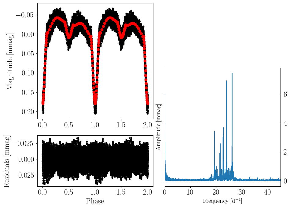
The residuals
Now that we’re confident that there’s some signal left over, lets see what we can do with it!
# Thanks, Dan Hey!
from echelle import interact_echelle
interact_echelle(nu_r[nu<=45], amp_r[nu<=45], dnu_min=0.1, dnu_max=10.)
/lhome/colej/software/miniconda3/envs/nominal3p9/lib/python3.9/site-packages/echelle-1.5.1-py3.9.egg/echelle/interact.py:201: UserWarning: You have multiple Jupyter servers open. You will need to pass the current notebook to `notebook_url`. i.e. interact_echelle(x,y,notebook_url='http://localhost:8888')